


- 1
- 2
- 3
- 4
- HFSS15�ھ�����
- ���
- HFSS�̌W
- HFSS 15 �ھ������ęn
HFSS Transient
Procedure for Viewing Transient Radiated Fields
To display transient radiated fields:
1. Add a radiation boundary. Radiated field calculations will only be done for designs with radiation boundaries.
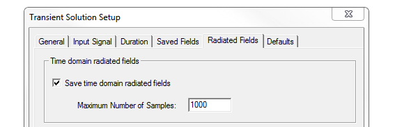
2. If a radiation boundary is present the transient Solve Setup contains the Radiated Fields tab with a "Save time domain radiated fields" checkbox. Select this option to make radiated fields available from a given setup. This applies to Transient with or without Network Analysis.
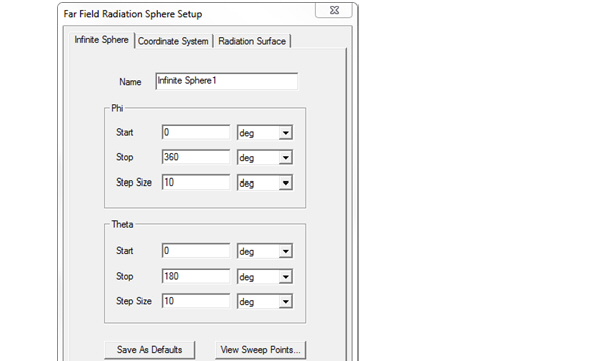
3. Under HFSS>Radiation, you can Insert Far Field Setup> Infinite Sphere. This menu is enabled for designs with radiation boundaries, even if no setups are saving radiated fields. The setup dialog resembles the one for frequency domain, but without the Radiation Surface tab. Use this dialog to set up the Theta and Phi sampling and, if needed, the local coordinate system. You can create multiple Infinite Sphere setups in a single design.
4. Once you have created a far field setup AND at least one setup has "Save radiated fields" selected, the Results menu will include Create Far Fields Report, with all submenus as in Frequency domain.
For Rectangular Plot, Rectangular Stacked Plot, and Data Table, the default is "Time" as the primary sweep, with Theta and Phi in Families set to single values corresponding to the first sample point.
For all other plots, the primary and secondary sweeps will be Theta and/or Phi, as in Frequency domain, and the Time is set to a single value - the start time.
5. In the Report dialog, the Solution selection includes only setups with "Save radiated fields" checked. The Geometry selection will include all far field Infinite Sphere setups. The Categories include rE, Variables, Output Variables, and Design. The rE quantities are as for frequency domain, but all quantities will be real.
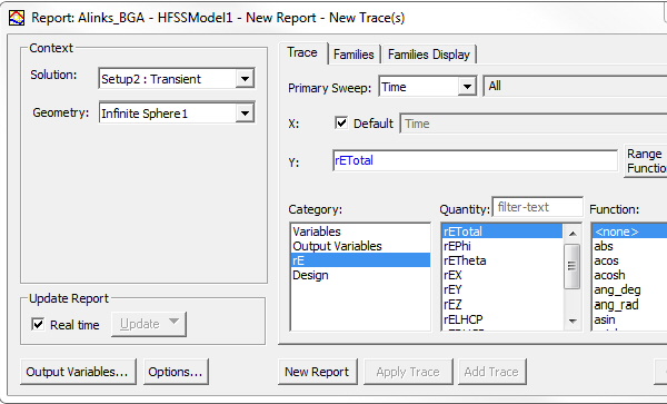
No matter what type of plot is generated, you can access the Time sweep and change the sampling, as with Field reports in Transient.
For 3D patterns, you can overlay the pattern on the geometry, and to animate versus time, as is done in frequency domain.
Once plots have been created, the reporter caches the base radiation field calculation. This means that subsequent plots will be generated more quickly. If you change the radiation setup, or invalidate solutions, the cache is cleared and the next plot takes longer.
For Transient Network Analysis, the radiated fields are based on the setup in Edit Sources. If you change the source excitations that forces recomputation of the radiated fields.
Output variables are supported, as for frequency domain.
Related Topics
HFSS Transient Getting Started Guides
Creating Reports
Plotting Field Overlays
-

������ȫ���HFSS��Ӗ�n�̣�����7��ҕ�l�̳̺�2���̲ģ��Y����v�⣬ҕ�l������ʾ���Y�����¹��̰�����HFSS�W�������y...��Ԕ����B��