久久精品视频免费,久久久久久久久免费视频,久久国产精品免费网站

Plotting in the Time Domain

The idea behind Time-Domain Reflectometry (TDR) is to excite a structure with a step function, and inspect the reflections as a function of time. Before you can examine the time domain, you must perform an Interpolating sweep for a driven solution (Modal or Terminal or Transient). You can then select Time from the Domain list in the Report dialog. You also need to specify the input signal, whether step or impulse.

With Time selected as the domain, you can select from several Categories and associated Quantities to plot, for example mag(S₁₁). When you plot in the Time domain, every frequency domain quantity is first converted to the time-domain before the formula is evaluated. For example, if you type in

S₁₁ / ( 1 - S₁₁ )

and plot it in the time domain the reporter will plot

IFFT(S₁₁ * input) / ( 1 - IFFT(S₁₁ * input) )

It will NOT plot

IFFT( S₁₁/ ( 1 - S₁₁) * input )

The two expressions are not equivalent.

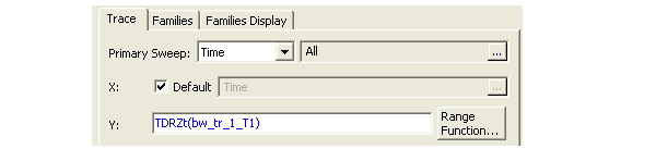
If you select Time Domain Impedance as the Category, you can select the TDRZ quantity. This is defined as

TDRZ(t) = Zref * ( 1 + IFFT(S₁₁ * input) ) / ( 1 - IFFT(S₁₁ * input) )

where "input" denotes the Fourier transform of the input signal (step or impulse) and "IFFT(.)" denotes the inverse FFT.

This equation is the instantaneous ratio of the time-domain voltage v(t) to the time-domain current i(t). That is because voltage and current are defined (in the frequency domain) in terms of the incident and reflected waves a and b, respectively, as

V = sqrt(Zo) * (a + b) = sqrt(Zo) * ( 1 + S_ii ) * a

I = 1/sqrt(Zo) * (a - b) = 1/sqrt(Zo) * ( 1 - S_ii ) * a

This lets the incident wave be the input step signal, and so when we take the inverse FFT of V and I, we get v(t) and i(t) in the time domain. Taking their ratio as a function of time then yields TDRZ(t). By default, Zo is equal to 50 Ohm.

To create a plot in the Time Domain:

1. For a design with an existing sweep setup, follow steps 1 - 4 for creating a report for design.

2. In the Report dialog box, in the Domain list, click Time.

This enables the TDR Options button and for terminal solution data reports includes the Terminal TDR Impedance in the Category list.

3. Click the TDR Options button.

The TDR Options dialog box appears.

4. Select the input signal type, Step or Impulse.

A Step describes a sustained change in the signal, whereas the Impulse is a brief excitation. Impulse is a very narrow rectangular pulse, with zero rise and fall time, width of 1 time step, and height of 1/(time step).

Selecting Step enables the Rise Time field, and Impulse disables it.

5. If you selected Step, enter the rise time of the pulse in the Rise Time text box.

The rise time should be appropriate for the frequency context.

With a band width from DC to f_max, the best time resolution that can be achieved is 1/(2f_max).

A rise time of 1/(2f_max) is the shortest rise time that can be resolved. However, a rise time of 0 s gives equally valuable information, so 0 is the default in this panel. See the example plot.

6. Enter the total time on the plot in the Maximum Plot Time text box.

The default maximum plot time in the TDR Options dialog is related to the delta frequency df in the frequency sweep: it is 1/2df, since that is the extent of time for which the IFFT gives information. This is often very long relative to the time delay that corresponds to the length of your device under test, so you may want to reduce this value. Alternatively, you can adjust the time axis of your TDR plot after it has been created.

7. Set the number of time points to plot in the Delta Time text box. By default, this is set to the number of points in the frequency sweep.

The delta time is based on the bandwidth of the sweep: with a frequency sweep from DC to f_max, the smallest time resolution you can obtain is given by 1/(2f_max). The IFFT algorithm provides data points as a spacing of 1/(2f_max), but you can smoothly interpolate between points by setting a finer resolution, e.g. to 1/(10f_max), at the expense of extra computation time.

8. Optionally, under TDR Window, modify the window type and width.

9. You can use the Save as Default to set the current values as a default, and the Use Defaults button to use previously saved options. Note that when you select a trace, the initial displayed values are those of the selected trace.

10. Click OK.

Optionally, to plot Terminal TDR impedance (that is, rather than calculate the S-parameter for waveport1 versus frequency, instead calculate the delay versus time at a particular impedance), do the following:

a. In the Category list, click Terminal TDR Impedance.

b. In the Quantity list, click a quantity to plot.

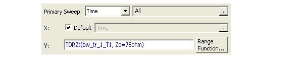
The default impedance (Zo) for the TDRZ quantity is 50 Ohms, unless you specified differently when you Set Renormalizing Impedance for Terminals when you created the terminals in the model. If you need a different impedance value, you can either edit the value in the Report dialog (as shown below), or you can create an Output Variable representing Zo × (1+S_ii)/(1-S_ii) with the Zo of your choice. To edit the Zo value in the Report dialog:

1. For the Category, select Terminal TDR Impedance, and the Port and Function of interest.

2. Edit the value by placing the cursor in the Value field.

In this example, the value for Zo is changed from the default to 75 Ohms by typing ‘,Zo=75ohm’ in the Y-column field.

c. In the Function list, click the mathematical function of the quantity to plot.

3. Click Done.

The report appears in the view window. It will be listed in the project tree.

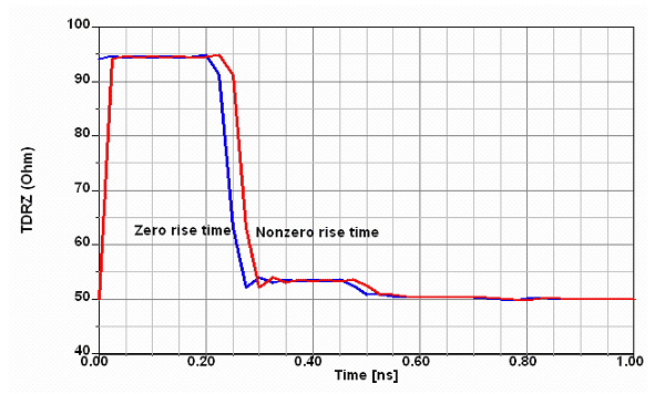
If S₁₁ = 0 at DC, the time-domain step response will settle to zero and the TDRZ step response settles to Zref. If S₁₁ is nonzero at DC, the time-domain step response will settle to a nonzero value and TDRZ will settle to a value different from Zref. The time-domain impulse response will always settle to zero, since it can be seen as the derivative of the step response. The TDRZ impulse response will always settle to Zref.

The plot below shows the difference between a short nonzero rise time and zero rise time for a transmission line segment of 94 Ohm. Note that the trace with zero rise time starts at the correct line impedance while the other starts at the renormalizing impedance. Other than that, one trace is a shifted version of the other. The reason the plot with finite rise time starts at 50 ohms is that the time-domain voltage and current are still at their steady state values, so v = Zref * i. As the pulse arrives, the TDRZ response changes from the steady-state behavior because there's a reflection from the transmission line back to the exciting source, which has a different renormalizing impedance from the characteristic impedance of the transmission line.

Some things to keep in mind with TDR:

(1)

where c is the speed of light in the medium and B is the bandwidth of the signal. Since TDR is usually based on a frequency band that starts at DC, the spatial resolution becomes

(2)

where F_max is the highest frequency in the frequency sweep. For example, if F_max = 15 GHz and the medium has e_r=4, the spatial resolution will be (1.5E8 m/s)/(3E10 /s) = 5 mm.

A spatial resolution of c/(2F_max) corresponds to a resolution in time

(3)

Let N be the number of points in the IFFT. N equals the number of time samples, and it also equals twice the number of frequency samples. The density of frequency samples in the frequency sweep influences the total time T as follows:

(4)

So increasing the density of the frequency samples leads to an increase in total time T. In practical case, this often leads to a long tail in the TDR plot with little useful information. Therefore, the TDR Options interface lets you set the maximum plot time to a smaller value.

The TDR Options interface also lets you choose a smaller Dt than given by equation (3) above. When you choose a smaller Dt, you increase F_max by "zero padding", i.e. adding zero values for S₁₁ beyond the calculated frequency sweep. Whether this is justified depends on your judgment. It leads in practice to a smoother TDR signal.

HFSS also lets you set the rise time of your input signal. The rise time should be at least 1/(2F_max). Even this rise time is a bit short for comfort, as it equals the duration of only one time sample. An input signal with a longer rise time has a smaller high-frequency content and will lead to reduced “ringing” in the TDR response.

A Hamming or Hann filter will also reduce the high-frequency content and tends to lead to a smoother TDR response. With these filters, one can select a width. A width of 100% is often a good choice.

Creating a report for design

TDR Windowing Functions

Perform TDR on Report


		Ansys HFSS，Ansoft HFSS online help，Version 15.0.	HFSS視頻教程 \| HFSS教程專欄 \| 射頻工程師培訓(xùn)培訓(xùn)課程 : Plotting in the Time Domain'>HFSSComments